Self-Replay Fine-Tuning: Extending Model Capabilities Made Simple
TL;DR Fine-tune a multimodal LLM on a narrow task and it usually forgets much of what it already knew. Self-Replay Fine-Tuning stops this by mixing filtered, model-generated general-domain responses into the training data. No change to the loss, the architecture, or the training loop. Across 4 models and 2 tasks††Models: MiniCPM-V-4.5, MiniCPM-o-4.5, GLM-4.1V, and Qwen3-VL-4B.
Tasks: Counting and Doc-OCR., it cuts forgetting by 80%+ while keeping essentially all of the task gain.
Fine-tuning is not always like adding a new book to a library. It can be more like writing new notes over an old page: the new lesson becomes clearer, but the words underneath begin to fade. Train a model intensively on one narrow task, and it may become much better at that task while losing language, reasoning, or visual abilities it once handled with ease. That trade-off is catastrophic forgetting (Figure 1).
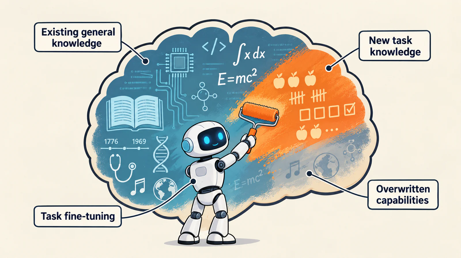
Fine-tuning a released multimodal LLM behaves the same way. Give it a clean supervised set and teach it to count objects in an image, and its counting accuracy shoots up. But re-run a general benchmark suite and the losses show up everywhere: OCR, instruction following, and output formatting all slip, and on the worst-hit models more than half of the general score disappears. The better the model gets at the narrow task, the more of its original ability it loses.
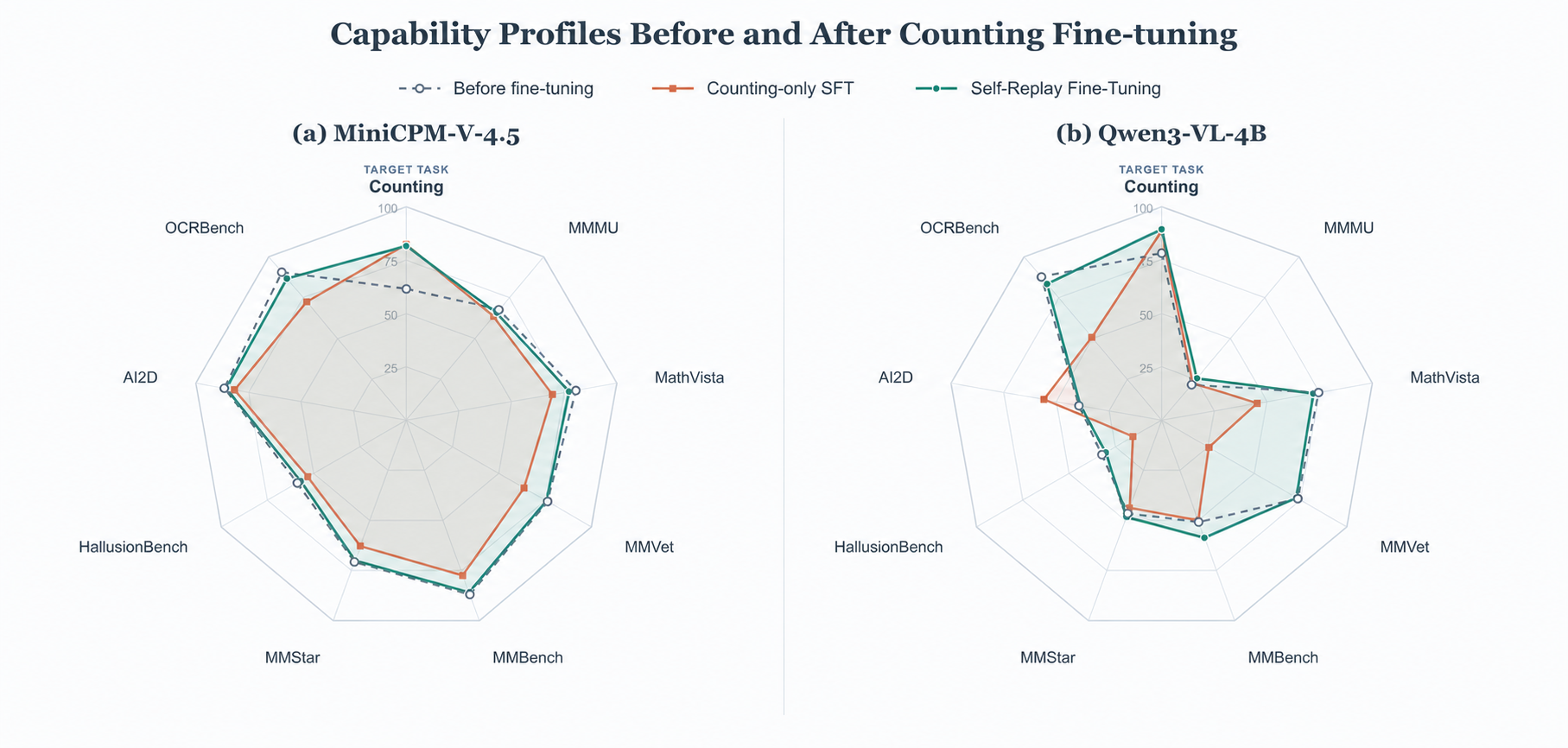
A broader capability view makes the trade-off concrete (Figure 2). For both MiniCPM-V-4.5 and Qwen3-VL-4B, counting-only SFT pushes the target Counting score outward while pulling several general capabilities inward. With Self-Replay Fine-Tuning, the models retain essentially the same Counting gain and recover a capability profile close to the one they had before fine-tuning.
This is catastrophic forgetting [1][1][1] McCloskey, M., & Cohen, N. J. (1989). Catastrophic interference in connectionist networks: The sequential learning problem. Psychology of Learning and Motivation, 24, 109–165.. Downstream SFT updates can overwrite capabilities acquired before fine-tuning, degrading general performance even as performance on the target task improves [2, 3][2, 3][2] Luo, Y., et al. (2023). An Empirical Study of Catastrophic Forgetting in Large Language Models During Continual Fine-tuning. arXiv preprint arXiv:2308.08747.[3] Li, H., et al. (2024). Revisiting Catastrophic Forgetting in Large Language Model Tuning. Findings of EMNLP 2024.. For a deployed model, that often means losing much of what made it useful in the first place.
The existing toolbox for fighting forgetting falls into four lines, and each comes with a real cost:
- Parameter regularization (EWC) [4][4][4] Kirkpatrick, J., et al. (2017). Overcoming catastrophic forgetting in neural networks. Proceedings of the National Academy of Sciences, 114(13), 3521–3526. penalizes drift from the initial weights, but the importance statistics are hard to estimate and calibrate at MLLM scale.
- Parameter isolation (LoRA) [5][5][5] Hu, E. J., et al. (2021). LoRA: Low-Rank Adaptation of Large Language Models. ICLR 2022. limits how much the weights can move, though that same ceiling can also cap task performance.
- Data replay [6][6][6] Rolnick, D., et al. (2019). Experience replay for continual learning. Advances in Neural Information Processing Systems, 32. mixes old-capability data into downstream fine-tuning, but the original training data may be private, unavailable, or impractical to retain. Public substitutes usually contain off-policy responses‡‡On-policy vs. off-policy: Here, “on-policy” describes label provenance: self-generated replay responses are sampled once from the pre-fine-tuning target checkpoint and remain fixed during SFT. Off-policy labels come from an external model or dataset., which are less effective at preserving the model's own pre-fine-tuning behavior.
- On-policy RL and distillation methods (e.g., GRPO and OPD) [7, 8][7, 8][7] Shao, Z., et al. (2024). DeepSeekMath: Pushing the Limits of Mathematical Reasoning in Open Language Models. arXiv preprint arXiv:2402.03300.[8] Lu, K. (2025). On-Policy Distillation. Thinking Machines Lab Technical Blog. optimize over the model's own rollouts. Their KL regularization or distillation objectives help constrain behavioral drift and mitigate forgetting. However, their on-policy updates cannot directly leverage high-quality offline SFT trajectories: learning relies on behaviors generated through the model's own exploration, while online rollout and scoring tightly couple data generation to training and carry high engineering cost.
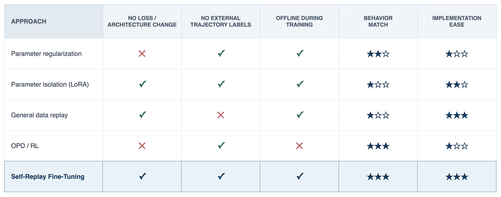
Our starting point is a simple question: how can we incorporate high-quality expert trajectories without compromising the model's existing capabilities? We let the model generate candidate responses to general prompts, retain high-quality and format-stable responses through rejection sampling, and mix them with the task data as ordinary SFT samples. We call this recipe Self-Replay Fine-Tuning. Because the replay labels come from the model itself, they better match its original response style and distribution. The method changes only the training data—no new objective, architecture, or custom training loop. The comparison below summarizes the practical trade-offs against other anti-forgetting approaches.
Anti-forgetting methods at a glance
Method
What we are optimizing
Every fine-tuning run trades off two quantities, and Self-Replay Fine-Tuning is built to move both in the right direction:
- Task Gain: how much the target-task metric improves after fine-tuning, relative to the original model.
- General Drop: how much the model's general ability falls, averaged over a suite of benchmarks it was not trained on.
Standard SFT usually buys Task Gain at the price of a large General Drop. The goal of Self-Replay Fine-Tuning is to keep Task Gain essentially intact while pushing General Drop close to zero. (Formal definitions and the exact metrics we report are in Appendix C.)
Generate, filter, remember
Self-Replay Fine-Tuning uses two separate data streams. The task dataset retains its original inputs and labels and provides supervision for learning the new task. Separately, general-domain inputs are passed through the pre-fine-tuning model to construct replay examples. After sampling and filtering, selected model-generated responses become the replay targets. These examples are then mixed with the unchanged task data for standard SFT. No task labels are replaced.
Replaying an off-the-shelf general corpus is like revising from a stranger's notes: the facts may be right, but they are written in a voice that is not yours, and drilling them can quietly overwrite your own habits. Self-Replay Fine-Tuning is closer to reviewing your own past work. Before fine-tuning, the model writes out answers to general prompts, we keep only the good ones, and we let it revisit those answers during training. Since the material already sounds like the model, rehearsing it reinforces its original behavior instead of disturbing it.
Concretely, Self-Replay Fine-Tuning consists of four offline replay-construction stages followed by standard mixed SFT (Figure 3).
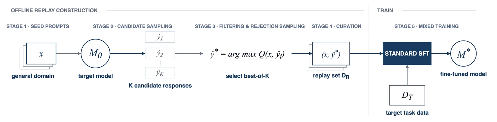
- Seed prompts. Collect prompts that span the model's original capabilities: general instructions, high-frequency business queries, preference and interaction data, and targeted subsets like OCR or VQA.
- Candidate sampling. For each prompt, the model that is about to be fine-tuned generates K candidate responses.
- Filtering and rejection sampling. Score candidates on factual correctness, format, length, safety, and chain-of-thought quality, then keep the best one that passes (best-of-K).
- Curation. Deduplicate, complete metadata, and balance the mix across capability buckets to get a clean, SFT-ready set.
- Mixed training. Blend the replay set into the task data at a Task:Replay ratio and run ordinary SFT.
View pseudocode
# 1. Seed prompts covering the model's original capabilities
prompts = load_seed_prompts()          # general chat, business, preference data, OCR/VQA, ...

# 2-3. Sample K candidates per prompt; keep the best one that passes every check
replay = []
for p in prompts:
    candidates = [model.generate(p, temperature=T) for _ in range(K)]
    passed = [c for c in candidates if quality_ok(c)]   # facts, format, length, safety, CoT
    if passed:
        replay.append((p, best_of(passed)))             # rejection sampling / best-of-K

# 4. Curate: dedup, fill metadata, balance across capability buckets
replay = curate(replay)

# 5. Mix with task data and run standard SFT. Nothing else changes.
train_data = task_data + alpha * replay
sft(model, train_data)
The first four stages run offline before training. The resulting replay set is then mixed with the task data for standard SFT. quality_ok and best_of are pluggable, so the same pipeline carries over across models and verifiers. Stage-by-stage details are in Appendix B.
Experiments
We run the main experiments on a Counting task (object counting, ~180K samples) across four models: MiniCPM-V-4.5, MiniCPM-o-4.5, GLM-4.1V, and Qwen3-VL-4B. Every setting shares identical hyperparameters and differs only in the data mix. Full setup is in Appendix C.
Forgetting drops by 80–99%, and task gain stays
Adding self-generated replay data at a 4:1 ratio§§Mixing ratio: Task:Replay = 4:1, so replay samples make up 20% of the mixed training set. cuts General Drop by 80–99% across all four models, while giving up less than 0.8 points of Task Gain (Figure 4a). Two cases stand out. GLM-4.1V, whose general score collapses from 75.5 to 32.2 under plain SFT, is almost fully restored to 73.1. Qwen3-VL-4B ends up slightly above its starting general score, a small positive transfer rather than a loss.
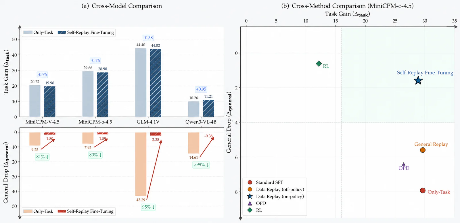
Table 2. Cross-model comparison of Self-Replay Fine-Tuning (Counting).
| Model | General Drop: Only-Task → Self-Replay | Forgetting reduced | Task Gain: Only-Task → Self-Replay |
|---|---|---|---|
| MiniCPM-V-4.5 | 9.25 → 1.80 | 81% | 20.72 → 19.96 |
| MiniCPM-o-4.5 | 7.92 → 1.59 | 80% | 29.66 → 28.90 |
| GLM-4.1V | 43.29 → 2.38 | 95% | 44.40 → 44.02 |
| Qwen3-VL-4B | 14.61 → −0.38 | >99% | 10.26 → 11.21 |
Those averages hide which specific skills break. On GLM-4.1V, counting-only SFT drops OCRBench (reading text in images) from 831 to 290, MMBench from 86 to 31, and MMVet (open-ended visual questions) from 68 to 22; Self-Replay Fine-Tuning brings them back to 833, 86, and 58.
These results establish that Self-Replay Fine-Tuning works consistently across models. We next ask whether it also offers a better task-retention trade-off than existing anti-forgetting approaches.
How Self-Replay Fine-Tuning compares to other anti-forgetting methods
We compare Self-Replay Fine-Tuning with OPD, RL, and off-policy replay on MiniCPM-o-4.5 + Counting, using the best configuration for each method.
Figure 4b shows that Self-Replay Fine-Tuning offers a favorable task–retention trade-off among the evaluated configurations, combining high task gain with low forgetting. The other evaluated configurations perform less favorably on at least one axis. OPD is very sensitive to initialization, ranging from ineffective (Task→Base learns almost nothing) to worse than plain SFT. RL preserves general ability but learns the task poorly. Off-policy general replay is the closest competitor, yet it still leaves about 3.5x more forgetting than Self-Replay Fine-Tuning.
Table 3. Cross-method comparison (MiniCPM-o-4.5, Counting). Best checkpoint for each method.¶¶Metrics: indicates general-capability degradation; means the retention benefit exceeds the task-performance cost.
| Method Category | Method | Task Acc | Δtask | General Score | Δgeneral | Net Gain |
|---|---|---|---|---|---|---|
| - | Baseline (zero-shot) | 55.70 | - | 77.58 | 0.00 | - |
| Standard SFT | Only-Task | 85.36 | 29.66 | 69.67 | 7.92 | - |
| OPD | Task→Base | 57.60 | 1.90 | 77.92 | −0.34 | −19.50 |
| Base→Task | 82.13 | 26.43 | 71.13 | 6.45 | −1.76 | |
| Mixed→Task | 79.66 | 23.96 | 69.16 | 8.42 | −6.21 | |
| RL | Binary reward | 66.54 | 10.84 | 77.40 | 0.18 | −11.09 |
| Continuous reward | 67.87 | 12.17 | 76.96 | 0.62 | −10.20 | |
| Data Replay | General (off-policy) | 85.36 | 29.66 | 72.00 | 5.59 | 2.33 |
| Self-Replay Fine-Tuning (on-policy) | 84.60 | 28.90 | 76.00 | 1.59 | 5.57 |
Highlights: blue marks positive transfer; green marks a favorable task–retention result; red marks the poorest result on a key comparison axis; underline marks the best Net Gain. OPD naming: "X→Y" denotes Teacher→Student. RL naming: Binary = 0/1 exact match; Continuous = 1 − |pred − gt| / gt.
Self-Replay Fine-Tuning achieves the strongest trade-off in this comparison, but the aggregate results do not reveal where that advantage comes from. We therefore turn to controlled ablations of the label source, replay ratio, and prompt source.
What drives the gains
The next three ablations examine the source of the labels, the replay ratio, and the source of the prompts. Together, the results are consistent with an important role for the model's own labels, beyond simply adding more general data. All ablations use MiniCPM-o-4.5 on Counting.
It is the on-policy labels, not just more general data
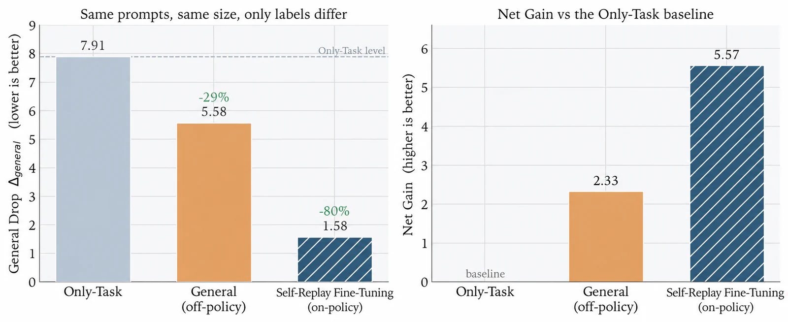
We hold the prompt set and the sample count fixed and change only the source of the labels: the model's own outputs (on-policy) versus the original open-source answers (off-policy). Everything else is identical.
Off-policy replay helps somewhat, bringing General Drop from 7.91 to 5.58. On-policy self-generated replay labels bring it down to 1.58, roughly an 80% reduction, at the same task accuracy (Figure 5). What matters is not adding general data, but adding data that matches the model's own pre-fine-tuning behavior.
A 4:1 mix achieves the highest Net Gain in our ratio sweep
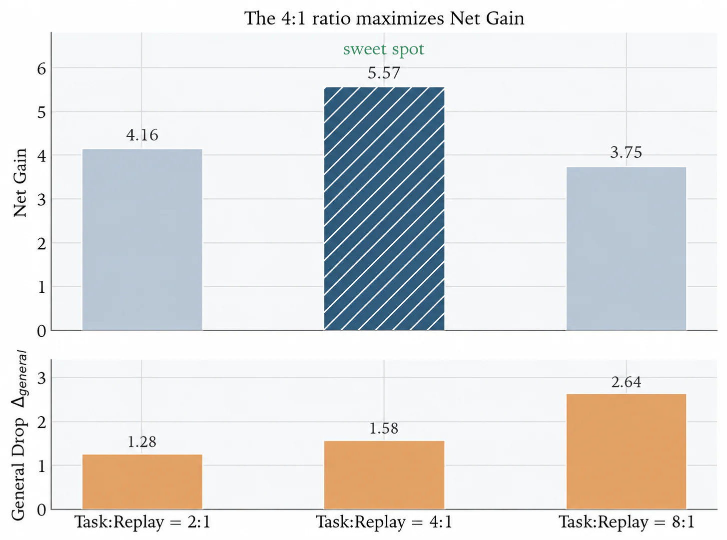
How much replay is enough? Fixing the Counting data and sweeping the Task:Replay ratio, Net Gain peaks at 4:1 (Figure 6). At 2:1 the extra replay starts to dilute task learning; at 8:1 there is too little replay to anchor the model and forgetting rises again. The 4:1 mix captures most of the anti-forgetting benefit at minimal task cost, so we use it as the default everywhere else.
The prompt source barely matters
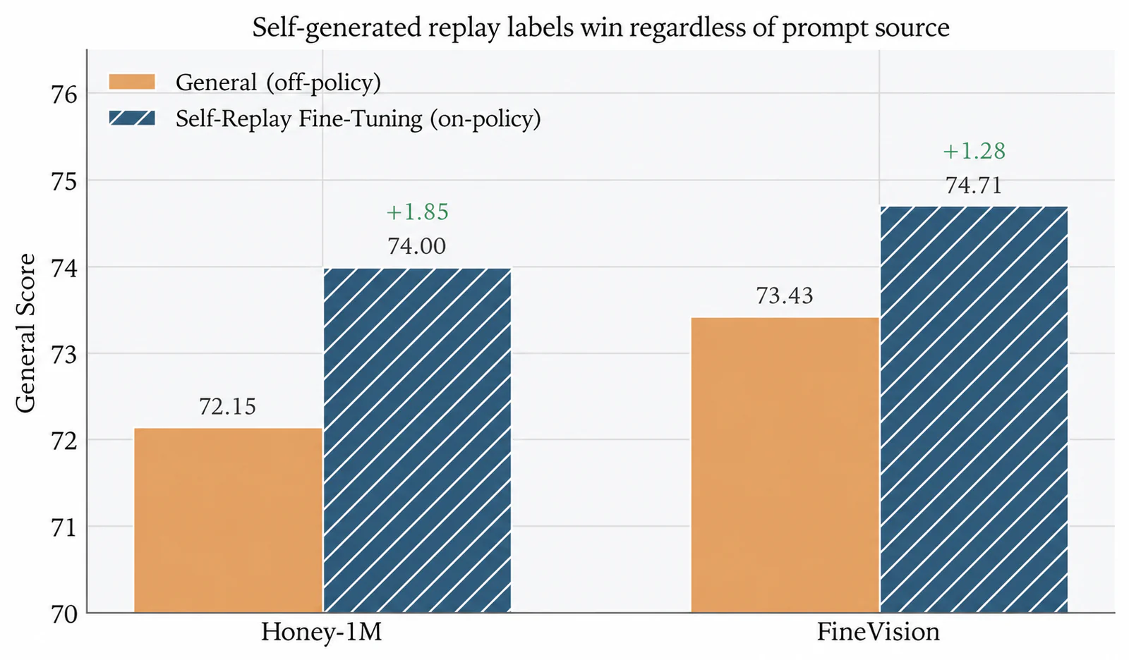
Could the gain simply come from a particularly favorable prompt set? To check, we swap the prompt source between two general corpora, Honey-1M and FineVision, and again compare self-generated replay labels against general labels. On both sources self-generated replay labels win by a similar margin, +1.85 and +1.28 General Score (Figure 7). The benefit tracks the label distribution, not the prompt origin, consistent with the hypothesis that the model's own labels are the key factor.
Beyond Counting
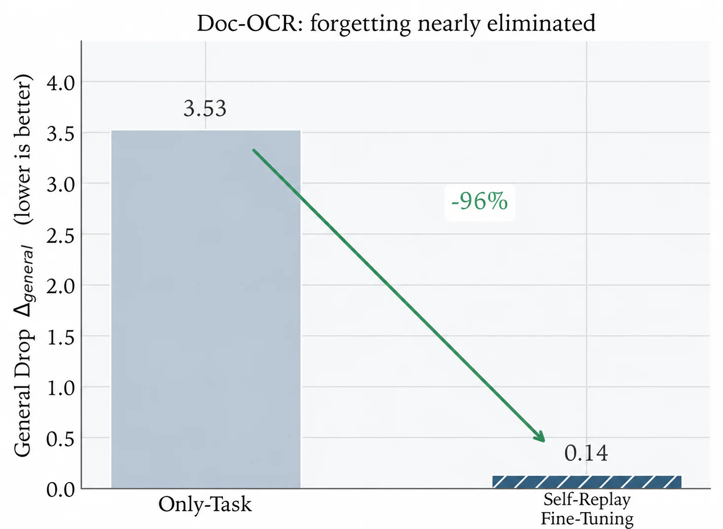
The ablations above identify what matters within Counting. We next ask whether the same recipe transfers to a different kind of task. We apply it to Doc-OCR on MiniCPM-V-4.5, a perception-heavy task very different from counting. Plain SFT costs 3.53 points of general ability; Self-Replay Fine-Tuning brings that down to 0.14, with task performance marginally better than Only-Task (Figure 8). The recipe is not tuned to Counting.
A production stress test
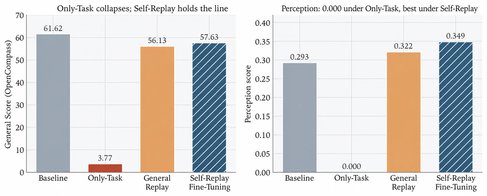
Benchmarks are one thing; a real deployment is another. We ran Self-Replay Fine-Tuning in a production setting, tracking the downstream task, a perception benchmark, and OpenCompass. Here plain SFT does not merely degrade, it collapses: the general score falls from 61.6 to 3.8, and perception drops to zero (Figure 9). Both replay strategies rescue the model, and Self-Replay Fine-Tuning comes out best on both fronts, with the highest perception score and the smallest general drop, while matching the others on task accuracy (all around 0.94).
Discussion
Why might Self-Replay Fine-Tuning help?
Replaying responses from the original checkpoint may give the model examples of its prior behavior to revisit while learning a new task. The label-source ablation supports this interpretation: with prompts and sample count held fixed, self-generated replay labels reduce General Drop to 1.58, compared with 5.58 for external labels, at matched task accuracy (Figure 5). This points to the choice of replay responses as an important factor in retention, alongside potential differences in response quality and content.
How often the model revisits these responses also matters. At a 2:1 Task:Replay ratio, replay yields the lowest General Drop but sacrifices more task gain; at 8:1, forgetting rises. The 4:1 setting achieves the highest Net Gain in the tested sweep (Figure 6). This suggests that preserving prior capabilities while learning the new task depends on balancing replay and task supervision. Increasing the replay share strengthens rehearsal but also changes how much training focuses on the new task.
The advantage also persists when the prompt corpus changes. Self-generated replay labels outperform external labels on both Honey-1M and FineVision, improving General Score by 1.85 and 1.28 points, respectively (Figure 7). Seeing the same direction of improvement across both sources makes the benefit less likely to be an artifact of one particular corpus and adds support for the role of the replay responses. The required breadth of prompt coverage remains unresolved.
The Doc-OCR result extends this picture beyond Counting. On MiniCPM-V-4.5, Self-Replay Fine-Tuning reduces General Drop from 3.53 to 0.14 while slightly improving the Doc-OCR task metric (Figure 8), showing a retention benefit in another model–task setting. These observations are consistent with a behavioral-anchor interpretation and recent evidence on on-policy data [9][9][9] Chen, H., Razin, N., Narasimhan, K., & Chen, D. (2025). Retaining by Doing: The Role of On-Policy Data in Mitigating Forgetting. arXiv preprint arXiv:2510.18874.. They measure retention outcomes and do not directly establish the underlying mechanism; broader task transfer still requires further evaluation.
Limitations and future directions
Self-Replay Fine-Tuning uses standard SFT without an added objective or model modification, but shifts work to offline sampling, filtering, and curation. Prompt coverage and response quality remain practical constraints: capabilities absent from the replay set receive no explicit rehearsal. The same set may be reusable across tasks when its coverage is appropriate, but the two-corpus comparison does not establish how much coverage is enough.
The main results cover Counting across four models, with additional Doc-OCR validation on one model and a production stress test. Broader task transfer remains to be established, and the 4:1 ratio is the best setting in the reported sweep, not a universal optimum.
We evaluate one fine-tuning round at a time. Regenerating replay responses from the current model between rounds is a possible extension, but a refreshed set could also reflect capability losses accumulated in earlier rounds. Future work should test long update sequences and compare refreshing the replay set with retaining examples from earlier checkpoints.
Conclusion
Self-Replay Fine-Tuning mitigates catastrophic forgetting at the data level. The model writes its own replay data, rejection sampling keeps the strongest responses, and those samples are mixed into the task data as ordinary SFT examples. Nothing in the loss, the architecture, or the training loop changes.
Across four models and two tasks, Self-Replay Fine-Tuning cuts forgetting by 80–99% while preserving essentially all of the task gain. In our comparison, the method offers a favorable task–retention trade-off among the evaluated configurations. The recurring lesson is simple: matching the model's own response distribution matters more than data volume. What saves the model is replaying data that already sounds like itself.
In practice, sample from the model, filter, mix in at roughly 4:1, and train as usual. Fine-tuning will always pull a model toward its new task. Self-Replay Fine-Tuning gives it something of its own to hold onto.
Appendix
A. Related work, briefly
Work on catastrophic forgetting in LLM and MLLM fine-tuning falls into four lines.
Parameter regularization (EWC, L2, KL constraints) [4][4] adds penalties that keep weights near the initial model. It needs no extra data, but it is hard to calibrate at scale, and estimating parameter importance such as Fisher information is expensive.
Parameter isolation (LoRA, adapters, layer freezing) [5][5] limits how many parameters can move. It is cheap to train, but low-rank updates can cap performance on multimodal tasks and add routing complexity in multi-task settings.
Data replay [6][6] mixes old-capability data into new training, but the original training data may be private, unavailable, or impractical to retain. Public substitutes typically contain off-policy responses that match the target model's behavior less closely. Later work moves toward self-generated data: SSR replays synthesized samples [10][10][10] Huang, J., et al. (2024). Mitigating Catastrophic Forgetting in Large Language Models with Self-Synthesized Rehearsal. Proceedings of ACL 2024., DMT stages the mixing [11][11][11] Dong, G., et al. (2024). How Abilities in Large Language Models are Affected by Supervised Fine-tuning Data Composition. Proceedings of ACL 2024., and SA-SFT stresses self-generated data for suppressing style drift [12][12][12] Sun, Y., et al. (2026). Talking to Yourself: Defying Forgetting in Large Language Models. arXiv preprint arXiv:2602.20162.. Lu (2025) also reports a closely related experiment that mixes fixed, self-generated background responses into document mid-training [8][8]. The common thread is that the source and label style of replay data matter more than sheer volume.
On-policy data. Data drawn from the model's own states narrows the train/inference gap and forgets less [9, 13][9, 13][13] Shenfeld, I., Damani, M., Hübotter, J., & Agrawal, P. (2026). Self-Distillation Enables Continual Learning. arXiv preprint arXiv:2601.19897.. OPD pushes this further with dense token-level teacher supervision on student rollouts [8][8], but tightly couples generation, scoring, and training.
Self-Replay Fine-Tuning sits between offline replay and fully online methods. It samples the model's own responses offline, filters them by rejection sampling, and then trains on them as ordinary SFT data. The expandable comparison in the introduction summarizes how it compares on the engineering dimensions that matter in practice.
B. Replay-data construction pipeline
This section gives the stage-by-stage details of the five-stage pipeline. Each stage is modular, so you can swap in different models or verifiers without changing the rest.
Stage 1: Seed Data Construction
First, we construct a set of prompts that broadly covers the model’s original capability distribution. The sources primarily include:
- General instructions: Post-training prompts covering basic dialogue and question-answering scenarios.
- High-frequency business queries: Frequent user instructions from real-world scenarios.
- Preference and interaction decision data: Data for optimizing response preferences, behavioral choices, and multi-step task execution.
- Targeted capability subsets: Vertical capabilities requiring focused preservation (e.g., OCR, VQA, document parsing, multi-turn dialogue).
Stage 2: Candidate Response Sampling
For each prompt , we use the model to be fine-tuned (or a closely related model from the same family) to generate candidate responses . This gives each prompt a pool of candidates for the next stage. We tune sampling temperature and decoding to balance diversity and quality; the sampling runs in parallel with checkpoint-resume for large batches.
Stage 3: Quality Filtering and Rejection Sampling
We apply multi-dimensional quality filtering to the candidate response set . The filtering criteria primarily cover:
- Factual correctness: Ensuring response content is consistent with objective facts or the given context.
- Format compliance: Verifying whether the output conforms to specific structural requirements (e.g., JSON format, specific answer tags).
- Length and redundancy control: Filtering out overly short meaningless responses or excessively long redundant outputs.
- Safety constraints: Removing samples containing harmful, biased, or out-of-bounds content.
- Chain-of-thought quality: For samples containing
<think>processes, detecting obvious hallucinations, logical discontinuities, or circular outputs.
When multiple candidates for the same prompt pass filtering, we apply a best-of- strategy to retain the response with the highest composite score, which essentially constitutes a rejection sampling process [14][14][14] Bai, Y., et al. (2022). Training a Helpful and Harmless Assistant with Reinforcement Learning from Human Feedback. arXiv preprint arXiv:2204.05862..
Stage 4: Replay Dataset Curation
The high-quality samples retained through rejection sampling must be aligned one-to-one with the original prompts and corresponding multimodal inputs, and formatted into the standard SFT training format, with the following cleanup:
- Deduplication and near-duplicate cleaning: Removing semantically highly redundant samples to avoid overfitting to specific patterns.
- Metadata completion: Ensuring each sample contains complete content while maintaining data traceability.
- Sampling balance: Up-sampling low-frequency categories or down-sampling high-frequency categories based on the distribution of capability subsets to maintain distributional uniformity.
The result is a clean training set that goes straight into the SFT pipeline.
Stage 5: Mixed Training
Finally, we mix the constructed self-generated replay data with the target task data at a preset ratio to form the training set and execute standard SFT. The mixing ratio (i.e., Task:Replay ratio) is the key hyperparameter controlling the trade-off between task adaptation and capability preservation, which we analyze in the ablations above.
C. Experimental setup
Tasks and Data
The main experiments are centered on the Counting (object counting) task, with the following setup:
- Downstream task: Counting (~180K training samples)
- Model pool: MiniCPM-V 4.5, MiniCPM-o 4.5, GLM-4.1V, Qwen3-VL-4B-Instruct
- Baselines: Only-Task, Task+General Data Replay, Self-Replay Fine-Tuning
- Core objective: Measure the trade-off between task gain and general-capability forgetting across the three data strategies
All experiments use identical training hyperparameters and vary only the data mixing strategy and ratio.
Evaluation Metrics
We use the following metrics across all experiments. Let and denote post-fine-tuning and zero-shot metric values respectively, and denote the OpenCompass composite score [15][15][15] OpenCompass Contributors. (2023). OpenCompass: A Universal Evaluation Platform for Foundation Models. arXiv preprint arXiv:2308.01893..
| Metric | Definition | Desired Direction |
|---|---|---|
| Task Metrics: core performance metric for the downstream task (e.g., Counting Acc) | ||
| OpenCompass general capability composite score, covering knowledge, reasoning, and language understanding | ||
| , where for higher-is-better metrics and for lower-is-better metrics | ||
| , i.e., General Drop | (positive = degradation) | |
| Net Gain: a composite metric measuring the net benefit relative to Only-Task |
General Drop is uniformly computed as “baseline OC minus post-fine-tuning OC,” so values closer to 0 are better; negative values indicate that post-fine-tuning general evaluation scores actually exceeded the initial model.
Net Gain is a composite evaluation metric we introduce to unify forgetting mitigation benefit and task performance cost into a single scalar for convenient cross-method comparison:
where the superscript OT denotes the Only-Task baseline. A Net Gain above 0 means the method mitigates more forgetting than the task performance it sacrifices, so higher is better.
Training Details
All baselines and ablations follow the same training setup. We introduce no additional loss terms, regularization constraints, or model architecture modifications; all models are fine-tuned with full parameters under identical hyperparameter configurations, differing only in training data composition (i.e., data mixing strategy and ratio).
Specifically, models are trained using the AdamW optimizer with a learning rate of , coupled with a cosine learning rate decay schedule with the first 5% of training steps used for warmup. Training is conducted on 8 NVIDIA A100 (80GB) GPUs with a per-device batch size of 1 and gradient accumulation steps of 16, yielding a global batch size of 128. To reduce memory overhead, we integrate DeepSpeed ZeRO-3 optimization.
Notes & References
Notes
- † Models: MiniCPM-V-4.5, MiniCPM-o-4.5, GLM-4.1V, and Qwen3-VL-4B.
Tasks: Counting and Doc-OCR.↩ - ‡ On-policy vs. off-policy: Here, “on-policy” describes label provenance: self-generated replay responses are sampled once from the pre-fine-tuning target checkpoint and remain fixed during SFT. Off-policy labels come from an external model or dataset.↩
- § Mixing ratio: Task:Replay = 4:1, so replay samples make up 20% of the mixed training set.↩
- ¶ Metrics: indicates general-capability degradation; means the retention benefit exceeds the task-performance cost.↩
References
- [1] McCloskey, M., & Cohen, N. J. (1989). Catastrophic interference in connectionist networks: The sequential learning problem. Psychology of Learning and Motivation, 24, 109–165.↩
- [2] Luo, Y., et al. (2023). An Empirical Study of Catastrophic Forgetting in Large Language Models During Continual Fine-tuning. arXiv preprint arXiv:2308.08747.↩
- [3] Li, H., et al. (2024). Revisiting Catastrophic Forgetting in Large Language Model Tuning. Findings of EMNLP 2024.↩
- [4] Kirkpatrick, J., et al. (2017). Overcoming catastrophic forgetting in neural networks. Proceedings of the National Academy of Sciences, 114(13), 3521–3526.↩
- [5] Hu, E. J., et al. (2021). LoRA: Low-Rank Adaptation of Large Language Models. ICLR 2022.↩
- [6] Rolnick, D., et al. (2019). Experience replay for continual learning. Advances in Neural Information Processing Systems, 32.↩
- [7] Shao, Z., et al. (2024). DeepSeekMath: Pushing the Limits of Mathematical Reasoning in Open Language Models. arXiv preprint arXiv:2402.03300.↩
- [8] Lu, K. (2025). On-Policy Distillation. Thinking Machines Lab Technical Blog.↩
- [9] Chen, H., Razin, N., Narasimhan, K., & Chen, D. (2025). Retaining by Doing: The Role of On-Policy Data in Mitigating Forgetting. arXiv preprint arXiv:2510.18874.↩
- [10] Huang, J., et al. (2024). Mitigating Catastrophic Forgetting in Large Language Models with Self-Synthesized Rehearsal. Proceedings of ACL 2024.↩
- [11] Dong, G., et al. (2024). How Abilities in Large Language Models are Affected by Supervised Fine-tuning Data Composition. Proceedings of ACL 2024.↩
- [12] Sun, Y., et al. (2026). Talking to Yourself: Defying Forgetting in Large Language Models. arXiv preprint arXiv:2602.20162.↩
- [13] Shenfeld, I., Damani, M., Hübotter, J., & Agrawal, P. (2026). Self-Distillation Enables Continual Learning. arXiv preprint arXiv:2601.19897.↩
- [14] Bai, Y., et al. (2022). Training a Helpful and Harmless Assistant with Reinforcement Learning from Human Feedback. arXiv preprint arXiv:2204.05862.↩
- [15] OpenCompass Contributors. (2023). OpenCompass: A Universal Evaluation Platform for Foundation Models. arXiv preprint arXiv:2308.01893.↩